What are the individual units that make up an image? Sure, one answer is pixels, each having a certain value. Another surprising one is sine functions with different parameters. In this article, I’ll convince you that any two-dimensional (2D) image can be reconstructed using only sine functions and nothing else. I’ll guide you through the code you can write to achieve this using the 2D Fourier transform in Python
I’ll talk about Fourier transforms. However, you don’t need to be familiar with this fascinating mathematical theory. I’ll describe the bits you need to know along the way. This will not be a detailed, technical tutorial about the Fourier transform, although if you’re here to learn about Fourier transforms and Fourier synthesis, then you’ll find this post useful to read alongside more technical texts.
Outline of This Article
The best way to read this article is from top to bottom. But if you’d like to jump across the sections, then here’s an outline of the article:
- Introduction: Every Image is Made Up of Only Sine Functions
- What are Sinusoidal Gratings?
- Creating Sinusoidal Gratings using NumPy in Python
- The Fourier Transform
- Calculating the 2D Fourier Transform of An Image in Python
- Reverse Engineering The Fourier Transform Data
- The Inverse Fourier Transform
- Finding All The Pairs of Points in The 2D Fourier Transform
- Using The 2D Fourier Transform in Python to Reconstruct The Image
- Conclusion
Who’s this article for?
-
Anyone wanting to explore using images in Python
-
Anyone who wants to understand 2D Fourier transforms and using FFT in Python
-
Those who are keen on optics and the science of imaging
-
Anyone who’s interested in image processing
-
Those with a keen interest in new Python projects, especially ones using NumPy
Every Image is Made Up of Only Sine Functions
Let me start by showing you the final result of this article. Let’s take an image such as this one showing London’s iconic Elizabeth Tower, commonly referred to as Big Ben. Big Ben is the name of the bell inside the tower, and not of the tower itself, but I digress:

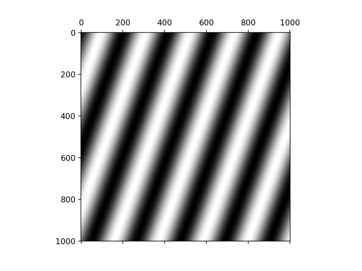
This image can be reconstructed from a series of sinusoidal gratings. A sinusoidal grating looks like this:

It’s called a sinusoidal grating because the grayscale values vary according to the sine function. If you plot the values along a horizontal line of the grating, you’ll get a plot of a sine function:

And here’s the reconstruction of the Elizabeth Tower image from thousands of different sinusoidal gratings:
Videos showing sinusoidal gratings and image reconstruction
In the video above and all other similar videos in this article:
- The image on the left shows the individual sinusoidal gratings
- The image on the right shows the sum of all the sinusoidal gratings
Therefore, each sinusoidal grating you see on the left is added to all the ones shown previously in the video, and the result at any time is the image on the right. Early on in the video, the image on the right is not recognisable. However, soon you’ll start to see the main shapes from the original image emerge. As the video goes on, more and more detail is added to the image. At the end of the video, the result is an image that’s identical to the original one.
The video shown above is sped up, and not all the frames are displayed. The final image has more than 90,000 individual sinusoidal gratings added together. In this article, you’ll use the 2D Fourier transform in Python to write code that will generate these sinusoidal gratings for an image, and you’ll be able to create a similar animation for any image you choose.
What Are Sinusoidal Gratings?
The sine function plots a wave. The wave described by the sine function can be considered to be a pure wave, and it has huge importance in all of physics, and therefore, in nature.
If you’re familiar with waves already, you can skip the next few lines and go straight to the discussion about sinusoidal gratings.
When dealing with waves, rather than simply using:
y=\sin(x)
you will usually use the following version:
y = \sin\left(\frac{2\pi x}{\lambda}\right)The term in the brackets represents an angle, and 
The term 


The wave can be better represented by:
y=A\sin\left(\frac{2\pi x}{\lambda}+\phi\right)

Sinusoidal gratings
A sinusoidal grating is a two-dimensional representation in which the amplitude varies sinusoidally along a certain direction. All the examples below are sinusoidal gratings having a different orientation:

There are other parameters that define a sinusoidal grating. You’ve seen these in the equation of the wave shown above. The amplitude of a sinusoidal grating, also referred to as contrast, determines the difference in grayscale values between the maximum and minimum points of a grating. Here are a few gratings with different amplitudes or contrasts:

In the grating with the highest amplitude, the peak of the grating is white, and the trough is black. When the amplitude is lower, the peak and trough are themselves levels of gray. If the amplitude is zero, as in the last example shown above, then there is no difference between the peak and the trough. The entire image has the same gray level. In this case, the contrast is zero, and there is no sine modulation left.
The next parameter that affects the grating is the wavelength or frequency. The shorter the length of the wave, the more waves fit in the same region of space, and therefore the frequency of the wave is higher. This is often referred to as spatial frequency. Below are examples of sinusoidal gratings with different wavelengths or frequencies:

From left to right, the wavelength is decreasing, and the frequency is increasing.
The final parameter is the phase of the grating. Two gratings can have the same frequency, amplitude and orientation, but not the same starting point. The gratings are shifted with respect to each other. Here are some examples of sinusoidal gratings with a different phase:


Ready to learn more NumPy – for free?
Get a week-long free pass to premium Python coding courses today, recorded by Stephen Gruppetta, author of The Python Coding Book. Includes a 3.5 hour NumPy course.
In summary, the parameters that describe a sinusoidal grating are:
- wavelength or frequency
- amplitude
- orientation
- phase
Creating Sinusoidal Gratings using NumPy in Python
Before I move on to talk about 2D Fourier transforms in Python, let’s create some sinusoidal gratings and see how you can vary the parameters I’ve just described. You won’t need to generate sinusoidal gratings directly in the rest of this article to deconstruct and then reconstruct an image using the 2D Fourier transform. Therefore, you can skip this section if you prefer to jump straight into Fourier transforms and Fourier synthesis. But if you’re not in a rush, this section will provide more insight into gratings and how to create them in Python.
In this article, I’ll use NumPy for all quantitative operations and Matplotlib for visualising. You’ll need to install these packages if you haven’t done so already.
Let’s create a 1D sine wave first before you move to the 2D version. The first script you’ll work on is called gratings.py:
# gratings.py

import numpy as np
import matplotlib.pyplot as plt

x = np.arange(-500, 501, 1)

wavelength = 200
y = np.sin(2 * np.pi * x / wavelength)

plt.plot(x, y)
plt.show()
You first create an array to represent the x-axis using np.arange(). You’re creating an array ranging from -500 to 500 with steps of 1. The endpoint is not included when using np.arange(), which is why 501 is used as the second argument. This array has 1001 elements. There’s a reason why I’m choosing an odd number of elements in the array. I’ll come back to this later.
You then define y using the simpler of the equations I discussed earlier. The wavelength is 200, which means that each wave will be 200 units long. This gives a sine wave when you plot it using plt.plot(). If you’re using an interactive environment, you won’t need to use the explicit call to plt.show(). However, all examples in this article are based on writing a script, so I’ll include the calls to plt.show() when required:

There are five waves present. This is what you’d expect since the wavelength is 200 units, and there are 1001 points in the array.
Moving from 1D sine to 2D sinusoidal grating
To translate this to a 2D grating, you’ll need to use np.meshgrid():
# gratings.py

import numpy as np
import matplotlib.pyplot as plt

x = np.arange(-500, 501, 1)

X, Y = np.meshgrid(x, x)

wavelength = 200
grating = np.sin(2 * np.pi * X / wavelength)

plt.set_cmap("gray")
plt.imshow(grating)
plt.show()
NumPy’s np.meshgrid() creates a 2D representation that can be used as the basis for 2D equations. I’m using capital X and Y to represent the 2D versions.
You can read more about meshgrid(), including alternatives that may be more efficient, in the article numpy.meshgrid(): How Does It Work? When Do You Need It? Are There Better Alternatives?
You change the colour map to grayscale before showing the image using plt.imshow(). This gives the following sinusoidal grating:
You can change the value of the variable wavelength to see how this affects the grating displayed. You can also replace X with Y to obtain a grating oriented along the vertical.
If you want to create a grating with any other orientation, you’ll need to transform the axes to account for rotation, for example:
# gratings.py

import numpy as np
import matplotlib.pyplot as plt

x = np.arange(-500, 501, 1)

X, Y = np.meshgrid(x, x)

wavelength = 200
angle = np.pi / 9
grating = np.sin(
    2*np.pi*(X*np.cos(angle) + Y*np.sin(angle)) / wavelength
)

plt.set_cmap("gray")
plt.imshow(grating)
plt.show()
You applied the rotation of axes transformation using 

As mentioned above, you won’t need to manually generate any sinusoidal gratings to deconstruct and then reconstruct images using 2D Fourier transforms in Python. You’ve seen how to change the frequency and orientation of gratings. I’ll leave it as an exercise for you to experiment with amplitude and phase if you wish.
The Python Coding Book is a relaxed and friendly programming textbook for beginners. Available in paperback and ebook editions.
The Fourier Transform
Now, it’s time for the star of the show. As I mentioned at the start, this is not a detailed tutorial on Fourier transforms, so I won’t dive into the maths of Fourier theory. Instead, I’ll focus on a general understanding of what they are and how they relate to images.
I will reverse the usual pattern of introducing a new concept and first show you how to calculate the 2D Fourier transform in Python and then explain what it is afterwards.
Using NumPy’s 2D Fourier transform functions
Let’s take the two sinusoidal gratings you created and work out their Fourier transform using Python’s NumPy. First, you can return to the one oriented along the horizontal axis by setting angle = 0:
# gratings.py

import numpy as np
import matplotlib.pyplot as plt

x = np.arange(-500, 501, 1)

X, Y = np.meshgrid(x, x)

wavelength = 200
angle = 0
grating = np.sin(
    2*np.pi*(X*np.cos(angle) + Y*np.sin(angle)) / wavelength
)

plt.set_cmap("gray")

plt.subplot(121)
plt.imshow(grating)

# Calculate Fourier transform of grating
ft = np.fft.ifftshift(grating)
ft = np.fft.fft2(ft)
ft = np.fft.fftshift(ft)

plt.subplot(122)
plt.imshow(abs(ft))
plt.xlim([480, 520])
plt.ylim([520, 480])  # Note, order is reversed for y
plt.show()
You use Matplotlib’s plt.subplot() to create two plots within the same figure. The function that calculates the 2D Fourier transform in Python is np.fft.fft2(). FFT stands for Fast Fourier Transform and is a standard algorithm used to calculate the Fourier transform computationally. There are other modules that provide the same functionality, but I’ll focus on NumPy in this article.
The lines immediately before and after the np.fft.fft2() call are important, but you can understand what’s happening without considering these two lines. Therefore, I’ll discuss them in an appendix for those who are interested and who want to go deeper with the 2D Fourier transform in Python.
The result of the FFT is an array of complex numbers. This is why you plot the absolute value of the Fourier transform ft, using the abs() built-in function. Note that you’re only doing this for the purposes of displaying the Fourier transform. You are not discarding the complex information from the array ft. You also zoom in to the central part of the image using plt.xlim() and plt.ylim() as that’s where all the action is. Note that the limits on the y-axis are reversed. This is due to how Matplotlib deals with displaying images and axes.
Understanding the Fourier Transform
The output from the code above is the following image:
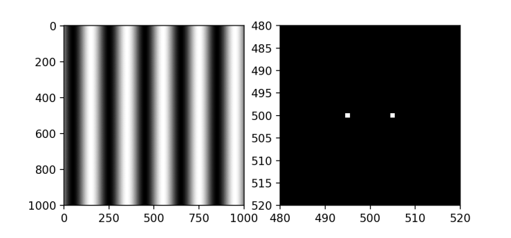
The sinusoidal grating on the left is the one you’ve seen earlier. On the right is the visual representation of the Fourier transform of this grating. It shows a value of 0 everywhere except for two points. Recall that the array is of size 1001 x 1001, and therefore, the centre of the array is (500, 500). The dots are at coordinates (495, 500) and (505, 500). They’re each five pixels away from the centre. You’ll see that they’re always symmetrical around the centre point.
This symmetry is the reason I chose to make the array dimensions odd. An array with odd dimensions has a single pixel that represents the centre, whereas when the dimensions are even, the centre is “shared” among four pixels:

Let’s see what happens if you double the frequency of the sinusoidal grating. To double the frequency, you half the wavelength:
# gratings.py

import numpy as np
import matplotlib.pyplot as plt

x = np.arange(-500, 501, 1)

X, Y = np.meshgrid(x, x)

wavelength = 100
angle = 0
grating = np.sin(
    2*np.pi*(X*np.cos(angle) + Y*np.sin(angle)) / wavelength
)

plt.set_cmap("gray")

plt.subplot(121)
plt.imshow(grating)

# Calculate Fourier transform of grating
ft = np.fft.ifftshift(grating)
ft = np.fft.fft2(ft)
ft = np.fft.fftshift(ft)

plt.subplot(122)
plt.imshow(abs(ft))
plt.xlim([480, 520])
plt.ylim([520, 480])  # Note, order is reversed for y
plt.show()
The output from this code is the following set of plots:

Each one of the two dots is now ten pixels away from the centre. Therefore, when you double the frequency of the sinusoidal grating, the two dots in the Fourier transform move further away from the centre.
The pair of dots in the Fourier transform represents the sinusoidal grating. Dots always come in symmetrical pairs in the Fourier transform.
Let’s rotate this sinusoidal grating by 20º, as you did earlier. That’s
# gratings.py

import numpy as np
import matplotlib.pyplot as plt

x = np.arange(-500, 501, 1)

X, Y = np.meshgrid(x, x)

wavelength = 100
angle = np.pi/9
grating = np.sin(
    2*np.pi*(X*np.cos(angle) + Y*np.sin(angle)) / wavelength
)

plt.set_cmap("gray")

plt.subplot(121)
plt.imshow(grating)

# Calculate Fourier transform of grating
ft = np.fft.ifftshift(grating)
ft = np.fft.fft2(ft)
ft = np.fft.fftshift(ft)

plt.subplot(122)
plt.imshow(abs(ft))
plt.xlim([480, 520])
plt.ylim([520, 480])  # Note, order is reversed for y
plt.show()
This gives the following set of sinusoidal grating and Fourier transform:

The dots are not perfect dots in this case. This is due to computational limitations and sampling, but it’s not relevant for this discussion, so I’ll ignore it here. You can read more about sampling and padding when using FFTs if you wish to go into more detail.
The Fourier Transform and The Grating Parameters
You’ll find that the distance of these dots from the centre is the same as in the previous example. The distance of the dots from the centre represents the frequency of the sinusoidal grating. The further the dots are from the centre, the higher the frequency they represent.
The orientation of the dots represents the orientation of the grating. You’ll find that the line connecting the dots to the centre makes an angle of 20º with the horizontal, same as the angle of the grating.
The other grating parameters are also represented in the Fourier transform. The value of the pixels making up the dots in the Fourier transform represents the amplitude of the grating. Information about the phase is encoded in the complex Fourier transform array, too. However, you’re displaying the absolute value of the Fourier transform. Therefore, the image you display doesn’t show the phase, but the information is still there in the Fourier transform array before you take the absolute value.
Therefore, the Fourier transform works out the amplitude, frequency, orientation, and phase of a sinusoidal grating.
Become a Member of
The Python Coding Place
Video courses, live cohort-based courses, workshops, weekly videos, members’ forum, and more…
Adding More Than One Grating
Let’s add two sinusoidal gratings together and see what happens. You add two gratings with different frequencies and orientations:
# gratings.py

import numpy as np
import matplotlib.pyplot as plt

x = np.arange(-500, 501, 1)

X, Y = np.meshgrid(x, x)

wavelength_1 = 200
angle_1 = 0
grating_1 = np.sin(
    2*np.pi*(X*np.cos(angle_1) + Y*np.sin(angle_1)) / wavelength_1
)
wavelength_2 = 100
angle_2 = np.pi/4
grating_2 = np.sin(
    2*np.pi*(X*np.cos(angle_2) + Y*np.sin(angle_2)) / wavelength_2
)

plt.set_cmap("gray")
plt.subplot(121)
plt.imshow(grating_1)
plt.subplot(122)
plt.imshow(grating_2)
plt.show()

gratings = grating_1 + grating_2

# Calculate Fourier transform of the sum of the two gratings
ft = np.fft.ifftshift(gratings)
ft = np.fft.fft2(ft)
ft = np.fft.fftshift(ft)

plt.figure()
plt.subplot(121)
plt.imshow(gratings)

plt.subplot(122)
plt.imshow(abs(ft))
plt.xlim([480, 520])
plt.ylim([520, 480])  # Note, order is reversed for y
plt.show()
The first figure you get with the first call of plt.show() displays the two separate sinusoidal gratings:

Note that if you’re running this in a script and not in an interactive environment, the program execution will pause when you call plt.show(), and will resume when you close the figure window.
You then add grating_1 to grating_2, and you calculate the Fourier transform of this new array which has two gratings superimposed on each other. The second figure displayed by this code shows the combined gratings on the left and the Fourier transform of this array on the right:

Although you cannot easily distinguish the two sinusoidal gratings from the combined image, the Fourier transform still shows the two components clearly. There are two pairs of dots which represent two sinusoidal gratings. One pair shows a grating oriented along the horizontal. The second shows a grating with a 45º orientation and a higher frequency since the dots are further from the centre.
Adding more sinusoidal gratings
Let’s go one step further and add more sinusoidal gratings:
# gratings.py

import numpy as np
import matplotlib.pyplot as plt

x = np.arange(-500, 501, 1)

X, Y = np.meshgrid(x, x)

amplitudes = 0.5, 0.25, 1, 0.75, 1
wavelengths = 200, 100, 250, 300, 60
angles = 0, np.pi / 4, np.pi / 9, np.pi / 2, np.pi / 12

gratings = np.zeros(X.shape)
for amp, w_len, angle in zip(amplitudes, wavelengths, angles):
    gratings += amp * np.sin(
        2*np.pi*(X*np.cos(angle) + Y*np.sin(angle)) / w_len
    )

# Calculate Fourier transform of the sum of the gratings
ft = np.fft.ifftshift(gratings)
ft = np.fft.fft2(ft)
ft = np.fft.fftshift(ft)

plt.set_cmap("gray")
plt.subplot(121)
plt.imshow(gratings)

plt.subplot(122)
plt.imshow(abs(ft))
plt.xlim([480, 520])
plt.ylim([520, 480])  # Note, order is reversed for y
plt.show()
You have now added the amplitude parameter, too. The amplitudes, wavelengths, and angles are now defined as tuples. You loop through these values using the zip() function. The array gratings needs to be initialised as an array of zeros before looping. You define this array to have the same shape as X.
The output of this code is the following figure:

The image on the left shows all five gratings superimposed. The Fourier transform on the right shows the individual terms as pairs of dots. The amplitude of the dots represents the amplitudes of the gratings, too.
You can also add a constant term to the final image. This is the background intensity of an image and is equivalent to a grating with zero frequency. You can add this simply by adding a constant to the image:
# gratings.py

import numpy as np
import matplotlib.pyplot as plt

x = np.arange(-500, 501, 1)

X, Y = np.meshgrid(x, x)

amplitudes = 0.5, 0.25, 1, 0.75, 1
wavelengths = 200, 100, 250, 300, 60
angles = 0, np.pi / 4, np.pi / 9, np.pi / 2, np.pi / 12

gratings = np.zeros(X.shape)
for amp, w_len, angle in zip(amplitudes, wavelengths, angles):
    gratings += amp * np.sin(
        2*np.pi*(X*np.cos(angle) + Y*np.sin(angle)) / w_len
    )

# Add a constant term to represent the background of image
gratings += 1.25

# Calculate Fourier transform of the sum of the gratings
ft = np.fft.ifftshift(gratings)
ft = np.fft.fft2(ft)
ft = np.fft.fftshift(ft)

plt.set_cmap("gray")
plt.subplot(121)
plt.imshow(gratings)

plt.subplot(122)
plt.imshow(abs(ft))
plt.xlim([480, 520])
plt.ylim([520, 480])  # Note, order is reversed for y
plt.show()
The Fourier transform shows this as a dot in the centre of the transform:

This is the only dot that doesn’t belong to a pair. The centre of the Fourier transform represents the constant background of the image.
Calculating The 2D Fourier Transform of An Image in Python
What’s the link between images and these sinusoidal gratings? Look back at the figure showing the array with five gratings added together. I’ll now claim that this is “an image”. An image, after all, is an array of pixels that each have a certain value. If we limit ourselves to grayscale images, then each pixel in an image is a value that represents the gray level of that pixel. Put these pixels next to each other and they reveal an image.
Now, the sum of five gratings doesn’t look like anything interesting. So let’s look at a real image, instead:

You can download this image of Earth, called "Earth.png" from the repository linked to this article:
There are also other images you’ll use later. You’ll need to place this image file in your project folder.
Reading The Image and Converting To Grayscale
To keep things a bit simpler, I’ll work in grayscale so that an image is a 2D array. Colour images are either 3D or 4D arrays. Some colour image formats are 3D arrays as they have a layer for red, one for green, and another for blue. Some image formats also have an alpha value which is a fourth layer. By converting colour images to grayscale, you can reduce them to a 2D array.
You’ll work on a new script called fourier_synthesis.py:
# fourier_synthesis.py

import matplotlib.pyplot as plt

image_filename = "Earth.png"

# Read and process image
image = plt.imread(image_filename)
image = image[:, :, :3].mean(axis=2)  # Convert to grayscale
print(image.shape)

plt.set_cmap("gray")

plt.imshow(image)
plt.axis("off")
plt.show()
You use Matplotlib’s plt.imread() to read the image into a NumPy array. Although there are better ways of converting a colour image into grayscale, the coarse method of averaging the red, green, and blue channels of the image is good enough for the purposes of this article. You’re discarding the information in the fourth alpha channel, if present. This gives a grayscale representation of the original image:
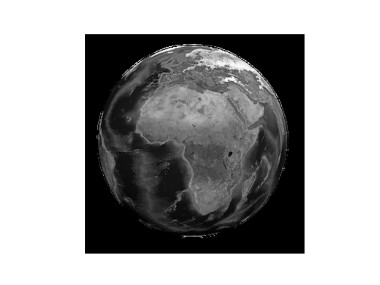
The printout of image.shape shows that this is a 301 x 301 pixel image. It’s already square and odd, which makes it easier to deal with. You’ll see later how you can deal with more general images.
Calculating the 2D Fourier Transform of The Image
You can work out the 2D Fourier transform in the same way as you did earlier with the sinusoidal gratings. As you’ll be working out the FFT often, you can create a function to convert an image into its Fourier transform:
# fourier_synthesis.py

import numpy as np
import matplotlib.pyplot as plt

image_filename = "Earth.png"

def calculate_2dft(input):
    ft = np.fft.ifftshift(input)
    ft = np.fft.fft2(ft)
    return np.fft.fftshift(ft)

# Read and process image
image = plt.imread(image_filename)
image = image[:, :, :3].mean(axis=2)  # Convert to grayscale

plt.set_cmap("gray")

ft = calculate_2dft(image)

plt.subplot(121)
plt.imshow(image)
plt.axis("off")
plt.subplot(122)
plt.imshow(np.log(abs(ft)))
plt.axis("off")
plt.show()
You calculate the 2D Fourier transform and show the pair of images: the grayscale Earth image and its transform. You display the logarithm of the Fourier transform using np.log() as this allows you to see what’s going on better. Without this change, the constant term at the centre of the Fourier transform would be so much brighter than all the other points that everything else will appear black. You’d be “blinded” by this one, central dot.
The output shows the following plots:

Now there are lots of dots that have non-zero values in the Fourier transform. Instead of five pairs of dots representing five sinusoidal gratings, you now have thousands of pairs of dots. This means that there are thousands of sinusoidal gratings present in the Earth image. Each pair of dots represents a sinusoidal grating with a specific frequency, amplitude, orientation, and phase. The further away the dots are from the centre, the higher the frequency. The brighter they are, the more prominent that grating is in the image as it has a higher amplitude. And the orientation of each pair of dots in relation to the centre represents the orientation of the gratings. The phase is also encoded in the Fourier transform.
Reverse Engineering The Fourier Transform Data
What do we know so far? The FFT algorithm in Python’s NumPy can calculate the 2D Fourier transform of the image. This decomposes the image into thousands of components. Each component is a sinusoidal grating.
If you take any matching pair of dots in the Fourier transform, you can extract all the parameters you need to recreate the sinusoidal grating. And if you do that for every pair of dots in the Fourier transform you’ll end up with the full set of gratings that make up the image.
Soon, you’ll see the code you can use to go through each pair of points in the Fourier transform. Before that, I need to add one more property of the Fourier transform that will make things a bit simpler.
The Inverse Fourier Transform
You are displaying the Fourier transform as a collection of pixels. It satisfies the definition of an “image”. So what would happen if you had to work out the Fourier transform of the Fourier transform itself? You’d end up with the original image!
There are a few technicalities that I’ll ignore here. For this reason, we use an inverse Fourier transform to get back to the original image, which is ever so slightly different from the Fourier transform. You can use NumPy’s np.fft.ifft2() to calculate an inverse Fourier transform.
Why is this useful? Because when you identify a pair of points in the Fourier transform, you can extract them from among all the other points and calculate the inverse Fourier transform of an array made up of just these two points and having the value zero everywhere else. This inverse Fourier transform will give the sinusoidal grating represented by these two points.
Let’s confirm this is the case with the gratings.py script you wrote earlier. You can go back to an early version where you had a single sinusoidal grating:
# gratings.py

import numpy as np
import matplotlib.pyplot as plt

x = np.arange(-500, 501, 1)

X, Y = np.meshgrid(x, x)

wavelength = 100
angle = np.pi/9
grating = np.sin(
    2*np.pi*(X*np.cos(angle) + Y*np.sin(angle)) / wavelength
)

plt.set_cmap("gray")

plt.subplot(131)
plt.imshow(grating)
plt.axis("off")

# Calculate the Fourier transform of the grating
ft = np.fft.ifftshift(grating)
ft = np.fft.fft2(ft)
ft = np.fft.fftshift(ft)

plt.subplot(132)
plt.imshow(abs(ft))
plt.axis("off")
plt.xlim([480, 520])
plt.ylim([520, 480])

# Calculate the inverse Fourier transform of
# the Fourier transform
ift = np.fft.ifftshift(ft)
ift = np.fft.ifft2(ift)
ift = np.fft.fftshift(ift)
ift = ift.real  # Take only the real part

plt.subplot(133)
plt.imshow(ift)
plt.axis("off")
plt.show()
There is an extra step to the code from earlier. You now work out the inverse Fourier transform of the Fourier transform you calculated from the original sinusoidal grating. The result should no longer be an array of complex numbers but of real numbers. However, computational limitations lead to noise in the imaginary part. Therefore, you only take the real part of the result.
The output of the above code is the following set of three plots:

The image on the right is the inverse Fourier transform of the image in the middle. This is the same grating as the original one on the left.
Finding All The Pairs of Points in The 2D Fourier Transform
Let’s jump back to the fourier_synthesis.py script and resume from where you left in the “Calculating The 2D Fourier Transform of An Image in Python” section. You can add a second function to calculate the inverse Fourier transform, and variables to store the size of the array and the index of the centre pixel:
# fourier_synthesis.py

import numpy as np
import matplotlib.pyplot as plt

image_filename = "Earth.png"

def calculate_2dft(input):
    ft = np.fft.ifftshift(input)
    ft = np.fft.fft2(ft)
    return np.fft.fftshift(ft)

def calculate_2dift(input):
    ift = np.fft.ifftshift(input)
    ift = np.fft.ifft2(ift)
    ift = np.fft.fftshift(ift)
    return ift.real

# Read and process image
image = plt.imread(image_filename)
image = image[:, :, :3].mean(axis=2)  # Convert to grayscale

# Array dimensions (array is square) and centre pixel
array_size = len(image)
centre = int((array_size - 1) / 2)

# Get all coordinate pairs in the left half of the array,
# including the column at the centre of the array (which
# includes the centre pixel)
coords_left_half = (
    (x, y) for x in range(array_size) for y in range(centre+1)
)

plt.set_cmap("gray")

ft = calculate_2dft(image)

plt.subplot(121)
plt.imshow(image)
plt.axis("off")
plt.subplot(122)
plt.imshow(np.log(abs(ft)))
plt.axis("off")
plt.show()
You also define coords_left_half. This generator yields pairs of coordinates that cover the entire left-hand half of the array. It also includes the central column, which contains the centre pixel. Since points come in pairs that are symmetrical around the centre point in a Fourier transform, you only need to go through coordinates in one half of the array. You can then pair each point with its counterpart on the other side of the array.
You’ll need to pay special attention to the middle column, but you’ll deal with this a bit later.
Sorting The Coordinates in Order of Distance From The Centre
When you start collecting the individual sinusoidal gratings to reconstruct the original image, it’s best to start with the gratings with the lowest frequencies first and progressively move through sinusoidal gratings with higher frequencies. You can therefore order the coordinates in coords_left_half based on their distance from the centre. You achieve this with a new function to work out the distance from the centre, calculate_distance_from_centre():
# fourier_synthesis.py

import numpy as np
import matplotlib.pyplot as plt

image_filename = "Earth.png"

def calculate_2dft(input):
    ft = np.fft.ifftshift(input)
    ft = np.fft.fft2(ft)
    return np.fft.fftshift(ft)

def calculate_2dift(input):
    ift = np.fft.ifftshift(input)
    ift = np.fft.ifft2(ift)
    ift = np.fft.fftshift(ift)
    return ift.real

def calculate_distance_from_centre(coords, centre):
    # Distance from centre is √(x^2 + y^2)
    return np.sqrt(
        (coords[0] - centre) ** 2 + (coords[1] - centre) ** 2
    )

# Read and process image
image = plt.imread(image_filename)
image = image[:, :, :3].mean(axis=2)  # Convert to grayscale

# Array dimensions (array is square) and centre pixel
array_size = len(image)
centre = int((array_size - 1) / 2)

# Get all coordinate pairs in the left half of the array,
# including the column at the centre of the array (which
# includes the centre pixel)
coords_left_half = (
    (x, y) for x in range(array_size) for y in range(centre+1)
)

# Sort points based on distance from centre
coords_left_half = sorted(
    coords_left_half,
    key=lambda x: calculate_distance_from_centre(x, centre)
)

plt.set_cmap("gray")

ft = calculate_2dft(image)

plt.subplot(121)
plt.imshow(image)
plt.axis("off")
plt.subplot(122)
plt.imshow(np.log(abs(ft)))
plt.axis("off")
plt.show()
The function calculate_distance_from_centre() takes a pair of coordinates and the index of the centre pixel as arguments and works out the distance of the point from the centre.
You use this function as the key for sorted(), which redefines the generator coords_left_half so that the points are in ascending order of distance from the centre. Therefore, the points represent increasing frequencies of the sinusoidal gratings.
Finding The Second Symmetrical Point in Each Pair
You have the points in the left half of the Fourier transform in the correct order. Now, you need to match them with their corresponding point on the other side of the 2D Fourier transform. You can write a function for this:
# fourier_synthesis.py

# ...

def find_symmetric_coordinates(coords, centre):
    return (centre + (centre - coords[0]),
            centre + (centre - coords[1]))
This function also needs two arguments: a set of coordinates and the index of the centre pixel. The function returns the coordinates of the matching point.
You’re now ready to work your way through all the pairs of coordinates. In the next section, you’ll start reconstructing the image from each individual sinusoidal grating.
Using the 2D Fourier Transform in Python to Reconstruct The Image
You’re ready for the home straight. The steps you’ll need next are:
- Create an empty array, full of zeros, ready to be used for each pair of points
- Iterate through the coordinates in
coords_left_half. For each point, find its corresponding point on the right-hand side to complete the pair - For each pair of points, copy the values of those points from the Fourier transform into the empty array
- Calculate the inverse Fourier transform of the array containing the pair of points. This gives the sinusoidal grating represented by these points
As you iterate through the pairs of points, you can add each sinusoidal grating you retrieve to the previous ones. This will gradually build up the image, starting from the low-frequency gratings up to the highest frequencies at the end:
# fourier_synthesis.py

import numpy as np
import matplotlib.pyplot as plt

image_filename = "Earth.png"

def calculate_2dft(input):
    ft = np.fft.ifftshift(input)
    ft = np.fft.fft2(ft)
    return np.fft.fftshift(ft)

def calculate_2dift(input):
    ift = np.fft.ifftshift(input)
    ift = np.fft.ifft2(ift)
    ift = np.fft.fftshift(ift)
    return ift.real

def calculate_distance_from_centre(coords, centre):
    # Distance from centre is √(x^2 + y^2)
    return np.sqrt(
        (coords[0] - centre) ** 2 + (coords[1] - centre) ** 2
    )

def find_symmetric_coordinates(coords, centre):
    return (centre + (centre - coords[0]),
            centre + (centre - coords[1]))

def display_plots(individual_grating, reconstruction, idx):
    plt.subplot(121)
    plt.imshow(individual_grating)
    plt.axis("off")
    plt.subplot(122)
    plt.imshow(reconstruction)
    plt.axis("off")
    plt.suptitle(f"Terms: {idx}")
    plt.pause(0.01)

# Read and process image
image = plt.imread(image_filename)
image = image[:, :, :3].mean(axis=2)  # Convert to grayscale

# Array dimensions (array is square) and centre pixel
array_size = len(image)
centre = int((array_size - 1) / 2)

# Get all coordinate pairs in the left half of the array,
# including the column at the centre of the array (which
# includes the centre pixel)
coords_left_half = (
    (x, y) for x in range(array_size) for y in range(centre+1)
)

# Sort points based on distance from centre
coords_left_half = sorted(
    coords_left_half,
    key=lambda x: calculate_distance_from_centre(x, centre)
)

plt.set_cmap("gray")

ft = calculate_2dft(image)

# Show grayscale image and its Fourier transform
plt.subplot(121)
plt.imshow(image)
plt.axis("off")
plt.subplot(122)
plt.imshow(np.log(abs(ft)))
plt.axis("off")
plt.pause(2)

# Reconstruct image
fig = plt.figure()
# Step 1
# Set up empty arrays for final image and
# individual gratings
rec_image = np.zeros(image.shape)
individual_grating = np.zeros(
    image.shape, dtype="complex"
)
idx = 0
# Step 2
for coords in coords_left_half:
    # Central column: only include if points in top half of
    # the central column
    if not (coords[1] == centre and coords[0] > centre):
        idx += 1
        symm_coords = find_symmetric_coordinates(
            coords, centre
        )
        # Step 3
        # Copy values from Fourier transform into
        # individual_grating for the pair of points in
        # current iteration
        individual_grating[coords] = ft[coords]
        individual_grating[symm_coords] = ft[symm_coords]

        # Step 4
        # Calculate inverse Fourier transform to give the
        # reconstructed grating. Add this reconstructed
        # grating to the reconstructed image
        rec_grating = calculate_2dift(individual_grating)
        rec_image += rec_grating

        # Clear individual_grating array, ready for
        # next iteration
        individual_grating[coords] = 0
        individual_grating[symm_coords] = 0

        display_plots(rec_grating, rec_image, idx)

plt.show()
You added one more function, display_plots(), which you use to display each individual sinusoidal grating and the reconstructed image. You use plt.pause(2) so that the first figure, which shows the image and its Fourier transform, is displayed for two seconds before the program resumes.
The main algorithm, consisting of the four steps listed above, works its way through the whole Fourier transform, retrieving sinusoidal gratings and reconstructing the final image. The comments in the code signpost the link between these steps and the corresponding sections in the code.
Speeding up the animation
This works. However, even for a small 301 x 301 image such as this one, there are 45,300 individual sinusoidal gratings. You’ll need to speed up the animation a bit. You can do this by displaying only some of the steps:
# fourier_synthesis.py

import numpy as np
import matplotlib.pyplot as plt

image_filename = "Earth.png"

def calculate_2dft(input):
    ft = np.fft.ifftshift(input)
    ft = np.fft.fft2(ft)
    return np.fft.fftshift(ft)

def calculate_2dift(input):
    ift = np.fft.ifftshift(input)
    ift = np.fft.ifft2(ift)
    ift = np.fft.fftshift(ift)
    return ift.real

def calculate_distance_from_centre(coords, centre):
    # Distance from centre is √(x^2 + y^2)
    return np.sqrt(
        (coords[0] - centre) ** 2 + (coords[1] - centre) ** 2
    )

def find_symmetric_coordinates(coords, centre):
    return (centre + (centre - coords[0]),
            centre + (centre - coords[1]))

def display_plots(individual_grating, reconstruction, idx):
    plt.subplot(121)
    plt.imshow(individual_grating)
    plt.axis("off")
    plt.subplot(122)
    plt.imshow(reconstruction)
    plt.axis("off")
    plt.suptitle(f"Terms: {idx}")
    plt.pause(0.01)

# Read and process image
image = plt.imread(image_filename)
image = image[:, :, :3].mean(axis=2)  # Convert to grayscale

# Array dimensions (array is square) and centre pixel
array_size = len(image)
centre = int((array_size - 1) / 2)

# Get all coordinate pairs in the left half of the array,
# including the column at the centre of the array (which
# includes the centre pixel)
coords_left_half = (
    (x, y) for x in range(array_size) for y in range(centre+1)
)

# Sort points based on distance from centre
coords_left_half = sorted(
    coords_left_half,
    key=lambda x: calculate_distance_from_centre(x, centre)
)

plt.set_cmap("gray")

ft = calculate_2dft(image)

# Show grayscale image and its Fourier transform
plt.subplot(121)
plt.imshow(image)
plt.axis("off")
plt.subplot(122)
plt.imshow(np.log(abs(ft)))
plt.axis("off")
plt.pause(2)

# Reconstruct image
fig = plt.figure()
# Step 1
# Set up empty arrays for final image and
# individual gratings
rec_image = np.zeros(image.shape)
individual_grating = np.zeros(
    image.shape, dtype="complex"
)
idx = 0

# All steps are displayed until display_all_until value
display_all_until = 200
# After this, skip which steps to display using the
# display_step value
display_step = 10
# Work out index of next step to display
next_display = display_all_until + display_step

# Step 2
for coords in coords_left_half:
    # Central column: only include if points in top half of
    # the central column
    if not (coords[1] == centre and coords[0] > centre):
        idx += 1
        symm_coords = find_symmetric_coordinates(
            coords, centre
        )
        # Step 3
        # Copy values from Fourier transform into
        # individual_grating for the pair of points in
        # current iteration
        individual_grating[coords] = ft[coords]
        individual_grating[symm_coords] = ft[symm_coords]

        # Step 4
        # Calculate inverse Fourier transform to give the
        # reconstructed grating. Add this reconstructed
        # grating to the reconstructed image
        rec_grating = calculate_2dift(individual_grating)
        rec_image += rec_grating

        # Clear individual_grating array, ready for
        # next iteration
        individual_grating[coords] = 0
        individual_grating[symm_coords] = 0

        # Don't display every step
        if idx < display_all_until or idx == next_display:
            if idx > display_all_until:
                next_display += display_step
                # Accelerate animation the further the
                # iteration runs by increasing
                # display_step
                display_step += 10
            display_plots(rec_grating, rec_image, idx)

plt.show()
You can adjust the parameters to speed up or slow down the reconstruction animation. In particular, you can use a smaller value for display_all_until. Note that in this code, I’m not choosing the fastest route, but one that focuses on undertanding the 2D Fourier transform in Python. Reconstructing each sinusoidal grating from a pair of points using the inverse Fourier Transform is time consuming. It is possible to extract the parameters of the grating from the values of this pair of points, and then generate the sinusoidal grating directly without using the inverse Fourier transform.
The output from this code is the video below:
The low-frequency components provide the overall background and general shapes in the image. You can see this in the sequence of the first few terms:

As more frequencies are added, more detail is included in the image. The fine detail comes in at the end with the highest frequencies. If you want to save the images to file, you can use plt.savefig().
Images Of Different Sizes
In the file repository, you’ll find a couple of other images to experiment with, and you can use your own images, too. You need to ensure that the image you use in the algorithm has an odd number of rows and columns, and it’s simplest to use a square image. You can add a bit more to fourier_synthesis.py to ensure that any image you load is trimmed down to a square image with odd dimensions:
# fourier_synthesis.py

import numpy as np
import matplotlib.pyplot as plt

image_filename = "Elizabeth_Tower_London.jpg"

def calculate_2dft(input):
    ft = np.fft.ifftshift(input)
    ft = np.fft.fft2(ft)
    return np.fft.fftshift(ft)

def calculate_2dift(input):
    ift = np.fft.ifftshift(input)
    ift = np.fft.ifft2(ift)
    ift = np.fft.fftshift(ift)
    return ift.real

def calculate_distance_from_centre(coords, centre):
    # Distance from centre is √(x^2 + y^2)
    return np.sqrt(
        (coords[0] - centre) ** 2 + (coords[1] - centre) ** 2
    )

def find_symmetric_coordinates(coords, centre):
    return (centre + (centre - coords[0]),
            centre + (centre - coords[1]))

def display_plots(individual_grating, reconstruction, idx):
    plt.subplot(121)
    plt.imshow(individual_grating)
    plt.axis("off")
    plt.subplot(122)
    plt.imshow(reconstruction)
    plt.axis("off")
    plt.suptitle(f"Terms: {idx}")
    plt.pause(0.01)

# Read and process image
image = plt.imread(image_filename)
image = image[:, :, :3].mean(axis=2)  # Convert to grayscale

# Array dimensions (array is square) and centre pixel
# Use smallest of the dimensions and ensure it's odd
array_size = min(image.shape) - 1 + min(image.shape) % 2

# Crop image so it's a square image
image = image[:array_size, :array_size]
centre = int((array_size - 1) / 2)

# Get all coordinate pairs in the left half of the array,
# including the column at the centre of the array (which
# includes the centre pixel)
coords_left_half = (
    (x, y) for x in range(array_size) for y in range(centre+1)
)

# Sort points based on distance from centre
coords_left_half = sorted(
    coords_left_half,
    key=lambda x: calculate_distance_from_centre(x, centre)
)

plt.set_cmap("gray")

ft = calculate_2dft(image)

# Show grayscale image and its Fourier transform
plt.subplot(121)
plt.imshow(image)
plt.axis("off")
plt.subplot(122)
plt.imshow(np.log(abs(ft)))
plt.axis("off")
plt.pause(2)

# Reconstruct image
fig = plt.figure()
# Step 1
# Set up empty arrays for final image and
# individual gratings
rec_image = np.zeros(image.shape)
individual_grating = np.zeros(
    image.shape, dtype="complex"
)
idx = 0

# All steps are displayed until display_all_until value
display_all_until = 200
# After this, skip which steps to display using the
# display_step value
display_step = 10
# Work out index of next step to display
next_display = display_all_until + display_step

# Step 2
for coords in coords_left_half:
    # Central column: only include if points in top half of
    # the central column
    if not (coords[1] == centre and coords[0] > centre):
        idx += 1
        symm_coords = find_symmetric_coordinates(
            coords, centre
        )
        # Step 3
        # Copy values from Fourier transform into
        # individual_grating for the pair of points in
        # current iteration
        individual_grating[coords] = ft[coords]
        individual_grating[symm_coords] = ft[symm_coords]

        # Step 4
        # Calculate inverse Fourier transform to give the
        # reconstructed grating. Add this reconstructed
        # grating to the reconstructed image
        rec_grating = calculate_2dift(individual_grating)
        rec_image += rec_grating

        # Clear individual_grating array, ready for
        # next iteration
        individual_grating[coords] = 0
        individual_grating[symm_coords] = 0

        # Don't display every step
        if idx < display_all_until or idx == next_display:
            if idx > display_all_until:
                next_display += display_step
                # Accelerate animation the further the
                # iteration runs by increasing
                # display_step
                display_step += 10
            display_plots(rec_grating, rec_image, idx)

plt.show()
The video you saw at the start of this article is the result of this code. There is also a third sample image in the file repository, which gives the following output:
You can now use any image with this code.
Final Words
Fourier transforms are a fascinating topic. They have plenty of uses in many branches of science. In this article, you’ve explored how the 2D Fourier transform in Python can be used to deconstruct and reconstruct any image. The link between the Fourier transform and images goes further than this, as it forms the basis of all imaging processes in the real world too, not just in dealing with digital images. Imaging systems from the human eye to cameras and more can be understood using Fourier Optics. The very nature of how light travels and propagates is described through the Fourier transform. But that’s a topic for another day!
The concepts you read about in this article also form the basis of many image processing tools. Some of the filtering done by image editing software use the Fourier transform and apply filtering in the Fourier domain before using the inverse Fourier transform to create the filtered image.
In this article, you’ve seen how any image can be seen as being made up of a series of sinusoidal gratings, each having a different amplitude, frequency, orientation, and phase. The 2D Fourier transform in Python enables you to deconstruct an image into these constituent parts, and you can also use these constituent parts to recreate the image, in full or in part.
Subscribe to
The Python Coding Stack
Regular articles for the intermediate Python programmer or a beginner who wants to “read ahead”
Read more of my Python articles at
The Python Coding Stack
Further Reading and References
- Read more about the Fourier Series and the Fourier Transform
- Learn more about NumPy in Chapter 8 of The Python Coding Book about using NumPy
- Find out more about the Fourier transform in the context of digital images and image processing in Gonzalez & Woods
- You’ve probably guessed that the name Fourier is the name of the person who first came up with the mathematical description of this principle. You can read about Joseph Fourier here.
- Image Credits:
- Elizabeth Tower London: Image by Lori Lo from Pixabay
- Earth illustration: Image by Arek Socha from Pixabay
- Malta Balconies: Image by Alex B from Pixabay
- One of the readers (see comments below) created a modified version of this code to work with RGB images which you can find here: https://github.com/Acelee2020/Visualization-of-2D-FFT-in-RGB
[This article uses KaTeX By Thomas Churchman]
Become a Member of
The Python Coding Place
Video courses, live cohort-based courses, workshops, weekly videos, members’ forum, and more…
Subscribe to
The Python Coding Stack
Regular articles for the intermediate Python programmer or a beginner who wants to “read ahead”
Appendix
Why is fftshift needed?
Look at one of the images you used in this article, such as the Elizabeth Tower picture. Where is the centre of the image? Seems like a silly question, no? However, when you represent an image as an array in Python, the pixel with indices (0, 0) is the one on the top right. This is the effective centre of the image from a mathematical viewpoint.
Now consider the images of the Fourier transforms you’ve seen above, where the centre of the image has significance, and the distance of points from this centre contains important information about the frequency of the sinusoidal gratings.
The np.fft.fftshift() and np.fft.ifftshif() functions take care of this. Let’s look at what np.fft.fftshift() does to a small array first:
>>> import numpy as np
>>> small_array = np.array([[1, 2, 3, 4],
...                         [5, 6, 7, 8],
...                         [9, 10, 11, 12],
...                         [13, 14, 15, 16]])
...
>>> small_array
array([[ 1,  2,  3,  4],
       [ 5,  6,  7,  8],
       [ 9, 10, 11, 12],
       [13, 14, 15, 16]])

>>> np.fft.fftshift(small_array)
array([[11, 12,  9, 10],
       [15, 16, 13, 14],
       [ 3,  4,  1,  2],
       [ 7,  8,  5,  6]])
The four quadrants are swapped so that the top left quadrant is now the bottom right one, and so on. This can be represented graphically with the following diagram:

What happens to the array if it has an odd number of rows and columns? Which quadrant should the centre row and column be considered in? This is the reason why there are two functions, an FFT shift and its inverse:
>>> small_array = np.array([[1, 2, 3, 4, 5],
...                         [6, 7, 8, 9, 10],
...                         [11, 12, 13, 14, 15],
...                         [16, 17, 18, 19, 20],
...                         [21, 22, 23, 24, 25]])
...
>>> small_array
array([[ 1,  2,  3,  4,  5],
       [ 6,  7,  8,  9, 10],
       [11, 12, 13, 14, 15],
       [16, 17, 18, 19, 20],
       [21, 22, 23, 24, 25]])

>>> np.fft.fftshift(small_array)
array([[19, 20, 16, 17, 18],
       [24, 25, 21, 22, 23],
       [ 4,  5,  1,  2,  3],
       [ 9, 10,  6,  7,  8],
       [14, 15, 11, 12, 13]])

>>> np.fft.ifftshift(small_array)  # Note the i in ifftshift
array([[13, 14, 15, 11, 12],
       [18, 19, 20, 16, 17],
       [23, 24, 25, 21, 22],
       [ 3,  4,  5,  1,  2],
       [ 8,  9, 10,  6,  7]])
Look at the all-important centre pixel, which has the value of 13 in the original array. One of the functions places this at the very end of the array (bottom right), whereas the other places it in the first position (top left).

Ready to learn more NumPy – for free?
Get a week-long free pass to premium Python coding courses today, recorded by Stephen Gruppetta, author of The Python Coding Book. Includes a 3.5 hour NumPy course.
[…] may find this article about using the 2D Fourier Transform in Python to reconstruct images from sine functions of interest, […]
The article says “It is possible to extract the parameters of the grating from the values of this pair of points, and then generate the sinusoidal grating directly”
I really want to konw how to extract the parameters of the grating from the values of the two points.
I want to know the parameters of the sin function.
I hope someone can solve my confusion, I would appreciate it!
Hello. Thank you for your comment. The rest of the article goes through the steps needed to do this. This is a central part of the technique used in this project. Each point of the FT is used to determine the amplitude, frequency, orientation and phase of the sinusoid it corresponds to. This section is probably the best one to look at: “Using the 2D Fourier Transform in Python to Reconstruct The Image”, but you’ll need to follow the rest of the article before it for this to make sense
Why using ifftshift before doing the fft calculation? I am wondering what the point of doing inverse first and then forward again. I tried without and the result seems to be less clean but roughly the same.
In some instances, this won’t make a difference, but in others it will have a small impact. The reason relates to how the phase component is dealt with in images that are odd x odd in size (examples 101 x 101). The central pixel is treated differently by fftshift and ifftshift and therefore the first ifftshift makes sure the central pixel becomes the top left pixel for the fft2, as required.
I’m planning to write a few more Fourier transform related posts and I’ll try to add more about this in those articles, with some examples
Still the functioning of ifftshift and fftshift is not clear to me. The appendix is too abstract.
I think maybe a more concrete example with comparison, formulas etc will make their functioning more transparent.
For now, I am using this as a black box, which is very uncomfortable.
I agree, using things as black boxes is very unsatisfying. I’ll be writing another post on Fourier Transforms in Python more generally (rather than specifically on decomposing images into sinusoidal gratings) and I’ll deal with what `fftshift` does, and why and when it’s needed, then.
It will also be better to show what are the ‘real frequencies’ of the transformed data. In your post, frequencies are the integer values, not the real frequencies. e.g if lambda=200, frequencies should be 0.005. Also, if the sample of x is not 1 between the neighboring sites, how does the transformed array represents the real frequency. It takes me some time to figure this out (experimentally), it will be best that a post with derivation to show how these elements are connected.
Lambda is the wavelength not the (spatial) frequency, though. The section labelled “What Are Sinusoidal Gratings?” introduces this concept briefly. The equations used use the wavelength as a parameter, which is a more natuaral parameter to use in these cases since it refers directly to the number of pixels covering one wave of the sinusoid. As you mention, the spatial frequency is the inverse of wavelength. So, lambda = 200 means that there are 200 pixels between peaks of a cycle, and that means that there are 0.005 cycles/pixel, which is the spatial frequency.
Excellent job! You probably don’t realize this, but you have basically described exactly how an east-west aligned aperture syntheis radio telescope works! What you call a ‘grating’ corresponds to the fringe pattern actually ‘seen’ by the telescope in the Fourier domain. Your images of ‘dots’ correspond to unresolved point sources in the image or sky domain.
Thanks Tony. I’m not that familiar with the details of synthetic radio telescopes, but I’m assuming there’s quite a bit of overlap with optical imaging. What I’m describing in the article is basically what happens in optical imaging systems, and the finite aperture of the system cuts off higher frequency terms, leading to diffraction. I assume this is the same underlying principle in radio telescopes (just a different part of the EM spectrum, after all)
In optical systems, you also have the issue of aberrations which attenuate some of the Fourier terms, leading to further loss of resolution.
[…] FFT, we first need to flatten this by converting it to grayscale. I found a useful tutorial here on ThePythonCodingBook. Ill add the code here for TL:DR […]
First of all, thank you for providing such an amazing program and resource available online for free. I recently undertook the task of doing a science project which involved using the Fourier transform for image processing, and I expanded on your code to make it work with an RGB image and show the process of the sine waves from each color channel being added up. I was wondering if I could have your permission to post the modified code onto GitHub for everyone to see and use, with credit to you as the original inspiration and as the author of most of the code of course. If not I understand
-Patrick
Hi Patrick. Absolutely, and let me know once you do so I can add a link to it on this article, too
Well here it is
https://github.com/Acelee2020/Visualization-of-2D-FFT-in-RGB
Not very efficient and not very pretty but it worked for my purposes
I have a question. In the past I have always used fftshift(fft(fftshift())) and fftshift(ifft(fftshift())) as fft and ifft. I have read your article, and you use fftshift(fft(ifftshift())) and fftshift(ifft(ifftshift())).
Which is the correct way to deal with it under normal circumstances? Does my previous approach cause problems for odd-numbered arrays or matrices?
It only makes a difference if you’re using the phase of the FFT. If you’re only using the amplitude/intensity, as in this tutorial, then it won’t make a difference. But in applications where you’re working with the real and imaginary components, it makes a difference I believe
Thank you for your answer. I tried fftshift(fft(fftshift())), fftshift(fft(ifftshift())), ifftshift(fft(fftshift())). When all three of them deal with the same odd array problem, the obtained phases are slightly different. I’m not sure which one is more correct?
The version I use is one I’ve been using for a very, very long time. I remember checking it at the time, but this was a very long time ago, so I’ll need to double check this. As most of the time it doesn’t matter, I haven’t bothered double checking this for decades…
[…] And to mark the 20th article of this new platform I revisited another special article from the past. The most popular article I’ve ever written by far—and one that ends up on Google’s first page often—is the August 2021 article on images and 2D Fourier transforms: How to Create Any Image Using Only Sine Functions | 2D Fourier Transform in Python. […]
Thanks for the article, you did really a great job! I read it with a lot of interest and I have some questions:
– about the `coords_left_half`. Why should be sorted and who and how will benefit of it? [Side remark: I think could be better to use a list comprehension with an in-place sort instead of using `sorted`]
– non-square image: a symmetry argumentation can still be used, right? Use a half image with diagonal & anti-diagonal symmetry to recover the full space of indices, would make sense? And for even*odd image? Just add a zero row or column?
– for a simple sine grading: the distance between two points in the magnitude space is the frequency, does a similar statement holds also in a frequency or phase space?
Thank you. Glad you enjoyed the article! The points in `coords_left_half` are sorted for display purposes. This way, when you reconstruct and create the video, the terms are added from low to high spatial frequency. It has no impact on the final result but affects the intermediate stages shown in the video. And yes, this would word for non-square images and even or odd images with some adjustments. I chose this to keep what’s already lengthy code and a a length article slightly more compact!
Thank you so much,I was recently working on a data set with many horizontal fringes, and I used the Fourier transform method. In this way, the data transformed into the frequency domain needs to be masked in the vertical direction of the central region. In this process, I found that once the most central point was masked (that is, its value was changed to 0), the image after inverse transformation could not be used at all, so the most central point must be excluded when masking. About Fourier transform, I did not know how to explain it to my teacher when I reported it. Although I still have some questions now, I understand a lot. Thank you for your excellent work!
Glad you enjoyed the article and found it useful! The central point in the Fourier domain represents the constant term—so, the uniform background (the average value of the whole image). So, if you remove it, the mean value will be shifted to zero