Do You Really Know What Sines and Cosines Are? Visualising Maths Using Python and Turtle

Sines and cosines are everywhere. But not everyone really understands what they are. In this article, you’ll write a Python program using the turtle module to visualise how they’re related to a circle. However, the take-home message goes beyond sines and cosines. It’s about visualising maths using Python code more generally.

Visualising mathematical relationships or scientific processes can help study and understand these topics. It’s a tool I’ve used a lot in my past working as a scientist. In fact, it’s one of the things that made me fall in love with programming.

Here’s the animation you’ll create by the end of this article:

How Are Sines and Cosines Linked to a Circle?

Before you dive into writing the code, let’s see why visualising maths using Python can be useful. In this case, you’re exploring one of the key building blocks of many areas of mathematics — sines and cosines.

You know what sin(x) and cos(x) look like. But how are they linked to the circle?

Look at the video above one more time…

The blue dot goes around the circumference of a circle at a constant angular speed. Its movement is smooth, and the dot doesn’t slow down or speed up.

Now, look at the yellow dot. Can you spot the connection between the yellow dot and the blue dot?

If you look carefully, you’ll notice that the yellow dot moves along a vertical line, up and down. Ignore the trace that seems to move out from the dot. Just focus on the dot for now.

The vertical position of the yellow dot tracks the blue dot’s vertical position. The yellow dot’s x-coordinate doesn’t change, but its y-coordinate is always the same as that of the blue dot.

Here’s the next thing to look out for. Is the speed of the yellow dot constant? Or does it speed up and slow down?

You’ve probably noticed that the yellow dot moves fastest when it’s in the middle of its up and down movement as it crosses the centre line. Then it slows down as it reaches the top or the bottom, changes direction and then accelerates towards the centre again.

This makes sense when you remember that the blue dot moves at a constant speed. When the yellow dot is at the top or the bottom, the blue dot moves mostly horizontally. Therefore the blue dot’s vertical movement is small or zero when it’s near the top and bottom of the circle.

The y-coordinate of the yellow dot is following sin(𝜃). The diagram below shows the angle 𝜃 :

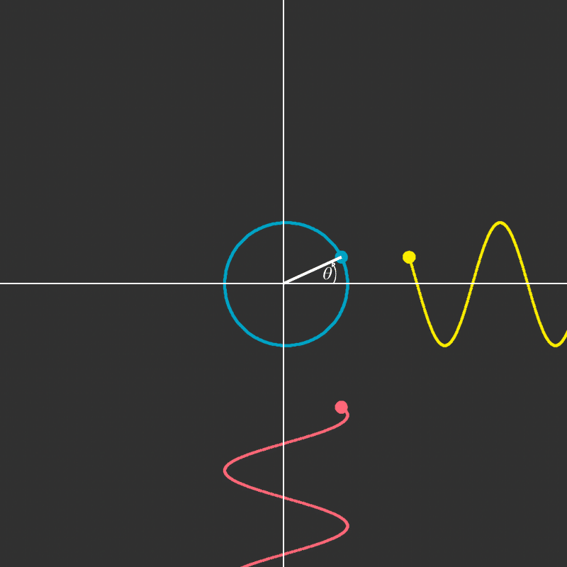
The angle is measured from the x-axis to the radius that connects the dot to the centre.

You can see the shape of the sine curve emerge from the trace that the yellow dot leaves.

I’ve discussed the yellow dot at length. How about the red dot? This dot is tracking the blue dot’s horizontal position. Its x-coordinate follows cos(𝜃).

Right, so if you’re only interested in visualising sines and cosines and how they’re related to the circle, then we’re done.

But if you’re also interested in visualising maths using Python, then read on…

Setting Up The Turtle Program

You’ll be using the turtle module in this program for visualising maths using Python. This module allows you to draw in a relatively straightforward way. It’s part of Python’s standard library, so you will already have this module on your computer if you’ve installed Python.

Don’t worry if you’ve never used this module before. I’ll explain the functions and methods you’ll use.

You can start by importing the module and creating your window where your animation will run:

import turtle

window = turtle.Screen()
window.bgcolor(50 / 255, 50 / 255, 50 / 255)

turtle.done()

The turtle.Screen() call creates an instance of the screen called window.

You also change its background colour. By default, turtle represents the red, green, and blue components of a colour as a float between 0 and 1. Although you can change the mode to use integers between 0 and 255, it’s just as easy to divide the RGB values by 255. We’ll go for a dark mode look in this animation!

The last line, turtle.done(), keeps the window open once the program has drawn everything else. Without this line, the program will terminate and close the window as soon as it reaches the end.

The main drawing object in the turtle module is turtle.Turtle(). You can move a turtle around the screen to draw. To draw the circle in the animation, you’ll need to create a turtle. You can also set a variable for the radius of the circle:

import turtle

radius = 100

window = turtle.Screen()
window.bgcolor(50 / 255, 50 / 255, 50 / 255)

main_dot = turtle.Turtle()
main_dot.pensize(5)
main_dot.shape("circle")
main_dot.color(0, 160 / 255, 193 / 255)
main_dot.penup()
main_dot.setposition(0, -radius)
main_dot.pendown()

turtle.done()

After creating the turtle, you change the “pen” size so that when the turtle draws lines later in the program, these lines will be thicker than the default value. You also change the shape of the turtle itself. You use the argument "circle" when using .shape(), which sets the shape of the turtle to a dot.

Next, you set the colour to blue and lift the pen up so that you can move the turtle to its starting position without drawing a line as the turtle moves. You keep the turtle at x=0 but change the y-coordinate to the negative value of the radius. This moves the dot downwards. This step ensures that the circle’s centre is at the centre of the window since, when you draw a circle, the dot will go around anticlockwise (counterclockwise).

When you run this code, you’ll see the blue dot on the dark grey background:

Going Around In A Circle

Next, you can make the dot go around in a circle. There are several ways you can achieve this using the turtle module. However, you’ll use the .circle() method here. This method has one required argument, radius, which determines the size of the circle.

You could write main_dot.circle(radius). However, this will draw the whole circle in one go. You want to break this down into smaller steps since you’ll need to perform other tasks at each position of this main dot.

You can use the optional argument extent in .circle(). This argument determines how much of the circle is drawn. Experiment with main_dot.circle(radius, 180), which draws a semi-circle, and then try other angles.

In this project, you can set a variable called angular_speed and then draw a small part of the circle in each iteration of a while loop:

import turtle

radius = 100
angular_speed = 2

window = turtle.Screen()
window.tracer(0)
window.bgcolor(50 / 255, 50 / 255, 50 / 255)

main_dot = turtle.Turtle()
main_dot.pensize(5)
main_dot.shape("circle")
main_dot.color(0, 160 / 255, 193 / 255)
main_dot.penup()
main_dot.setposition(0, -radius)
main_dot.pendown()

while True:
    main_dot.circle(radius, angular_speed)

    window.update()

turtle.done()

The dot will draw a small arc of the circle in each iteration of the while loop. Since you set angluar_speed to 2, the turtle will draw 2º of the circle in each iteration.

You’ve also set window.tracer(0) as soon as you create the window. This stops every step each turtle makes from being drawn on the screen. Instead, it gives you control over when to update the screen. You add window.update() at the end of the while loop to update the screen once every iteration. One iteration of the loop is equivalent to one frame of the animation.

Using window.tracer(0) and window.update() gives you more control over the animation and also speeds up the drawing, especially when the program needs to draw lots of things.

When you run the code, you’ll see the dot going around in a circle:

Don’t worry about the speed of the dot at this stage. You’ll deal with the overall speed of the animation towards the end when you have everything else already in place. However, you can use a smaller value for angular_speed if you want to slow it down.

Tracking The Blue Dot’s Vertical Motion

You can now create another turtle which will track the blue dot’s vertical motion. You’ll make this dot yellow and shift it to the right of the circle:

import turtle

radius = 100
angular_speed = 2

window = turtle.Screen()
window.tracer(0)
window.bgcolor(50 / 255, 50 / 255, 50 / 255)

main_dot = turtle.Turtle()
main_dot.pensize(5)
main_dot.shape("circle")
main_dot.color(0, 160 / 255, 193 / 255)
main_dot.penup()
main_dot.setposition(0, -radius)
main_dot.pendown()

vertical_dot = turtle.Turtle()
vertical_dot.shape("circle")
vertical_dot.color(248 / 255, 237 / 255, 49 / 255)
vertical_dot.penup()
vertical_dot.setposition(
    main_dot.xcor() + 2 * radius,
    main_dot.ycor(),
)

while True:
    main_dot.circle(radius, angular_speed)

    vertical_dot.sety(main_dot.ycor())

    window.update()

turtle.done()

You set vertical_dot‘s initial position by using the position of main_dot as reference. The methods main_dot.xcor() and main_dot.ycor() return the x- and y- coordinates of the turtle when they’re called. If you choose to move the circle to a different part of the screen, vertical_dot will move with it since you’re linking vertical_dot‘s position to main_dot.

You add 2 * radius to main_dot‘s x-coordinate so that vertical_dot is always twice as far from the centre of the circle as the circle’s circumference on the x-axis.

In the while loop, you change vertical_dot‘s y-coordinate using vertical_dot.sety(). This dot tracks main_dot‘s y-coordinate, which means that main_dot and vertical_dot will always have the same height on the screen.

You can see the yellow dot tracking the blue dot’s vertical position when you run this code:

Incidentally, you can also remove the turtle.done() call at the end of the code now since you have an infinite loop running, so the program will never terminate. I’ll remove this call in the next code snippet.

Tracking The Blue Dot’s Horizontal Motion

You can follow the same pattern above to track the blue dot’s horizontal motion. In this case, you can set the dot’s colour to red and place it below the circle:

import turtle

radius = 100
angular_speed = 2

window = turtle.Screen()
window.tracer(0)
window.bgcolor(50 / 255, 50 / 255, 50 / 255)

main_dot = turtle.Turtle()
main_dot.pensize(5)
main_dot.shape("circle")
main_dot.color(0, 160 / 255, 193 / 255)
main_dot.penup()
main_dot.setposition(0, -radius)
main_dot.pendown()

vertical_dot = turtle.Turtle()
vertical_dot.shape("circle")
vertical_dot.color(248 / 255, 237 / 255, 49 / 255)
vertical_dot.penup()
vertical_dot.setposition(
    main_dot.xcor() + 2 * radius,
    main_dot.ycor(),
)

horizontal_dot = turtle.Turtle()
horizontal_dot.shape("circle")
horizontal_dot.color(242 / 255, 114 / 255, 124 / 255)
horizontal_dot.penup()
horizontal_dot.setposition(
    main_dot.xcor(),
    main_dot.ycor() - radius,
)

while True:
    main_dot.circle(radius, angular_speed)

    vertical_dot.sety(main_dot.ycor())

    horizontal_dot.setx(main_dot.xcor())

    window.update()

You set horizontal_dot‘s initial position at a distance equal to the radius lower than main_dot. Recall that the blue dot starts drawing the circle from its lowest point. In the while loop, horizontal_dot is tracking main_dot‘s x-coordinate. Therefore, the blue and red dots are always sharing the same position along the x-axis.

The animation now has both yellow and red dots tracking the blue dot:

You can already see that although the blue dot is moving at a constant speed around the circumference of the circle, the yellow and red dots are speeding up and slowing down as they move.

You can stop here. Or you can read further to add a trace to the yellow and red dots to show how their speed is changing in more detail.

Adding A Trace To The Yellow and Red Dots

Next, you’ll get the yellow and red dots to leave a mark on the drawing canvas in each loop iteration. These marks will then move outwards to make way for the new marks drawn by the dots in the next iteration.

Let’s focus on the yellow dot first. You can create a new turtle by cloning vertical_dot and hiding the actual turtle. You can then create a set of x-values to represent all the points between the x-position of the yellow dot and the right-hand side edge of the window:

import turtle

radius = 100
angular_speed = 2

window = turtle.Screen()
window.tracer(0)
window.bgcolor(50 / 255, 50 / 255, 50 / 255)

main_dot = turtle.Turtle()
main_dot.pensize(5)
main_dot.shape("circle")
main_dot.color(0, 160 / 255, 193 / 255)
main_dot.penup()
main_dot.setposition(0, -radius)
main_dot.pendown()

vertical_dot = turtle.Turtle()
vertical_dot.shape("circle")
vertical_dot.color(248 / 255, 237 / 255, 49 / 255)
vertical_dot.penup()
vertical_dot.setposition(
    main_dot.xcor() + 2 * radius,
    main_dot.ycor(),
)

vertical_plot = vertical_dot.clone()
vertical_plot.hideturtle()
start_x = int(vertical_plot.xcor())
# Get range of x-values from position of dot to edge of screen
x_range = range(start_x, window.window_width() // 2 + 1)
# Create a list to store the y-values to draw at each
# point in x_range.
vertical_values = [None for _ in x_range]
# You can populate the first item in this list
# with the dot's starting height
vertical_values[0] = vertical_plot.ycor()

horizontal_dot = turtle.Turtle()
horizontal_dot.shape("circle")
horizontal_dot.color(242 / 255, 114 / 255, 124 / 255)
horizontal_dot.penup()
horizontal_dot.setposition(
    main_dot.xcor(),
    main_dot.ycor() - radius,
)

while True:
    main_dot.circle(radius, angular_speed)

    vertical_dot.sety(main_dot.ycor())

    horizontal_dot.setx(main_dot.xcor())

    window.update()

The variable x_range stores all the points from the x-position of the yellow dot to the edge of the screen. In this example, I’m using all the pixels. However, you can use the optional argument step when using range() if you prefer to use a subset of these points, for example, one out of every two pixels. Using fewer points can speed up the animation if it becomes too sluggish, but it will also change the frequency of the sine curve that the animation displays.

You also created the list vertical_values whose length is determined by the number of points in x_range. Each item in this list will contain the y-coordinate that needs to be plotted. All these values are set to None initially except for the first item.

The blue dot will move in each iteration in the while loop. Therefore, so will the yellow dot. Next, you need to register the new y-coordinate of the yellow dot in the vertical_values list. However, first, you’ll need to move all the existing values forward. The first item becomes the second, the second item becomes the third, and so on.

Let’s try this approach first:

import turtle

radius = 100
angular_speed = 2

window = turtle.Screen()
window.tracer(0)
window.bgcolor(50 / 255, 50 / 255, 50 / 255)

main_dot = turtle.Turtle()
main_dot.pensize(5)
main_dot.shape("circle")
main_dot.color(0, 160 / 255, 193 / 255)
main_dot.penup()
main_dot.setposition(0, -radius)
main_dot.pendown()

vertical_dot = turtle.Turtle()
vertical_dot.shape("circle")
vertical_dot.color(248 / 255, 237 / 255, 49 / 255)
vertical_dot.penup()
vertical_dot.setposition(
    main_dot.xcor() + 2 * radius,
    main_dot.ycor(),
)

vertical_plot = vertical_dot.clone()
vertical_plot.hideturtle()
start_x = int(vertical_plot.xcor())
# Get range of x-values from position of dot to edge of screen
x_range = range(start_x, window.window_width() // 2 + 1)
# Create a list to store the y-values to draw at each
# point in x_range.
vertical_values = [None for _ in x_range]
# You can populate the first item in this list
# with the dot's starting height
vertical_values[0] = vertical_plot.ycor()

horizontal_dot = turtle.Turtle()
horizontal_dot.shape("circle")
horizontal_dot.color(242 / 255, 114 / 255, 124 / 255)
horizontal_dot.penup()
horizontal_dot.setposition(
    main_dot.xcor(),
    main_dot.ycor() - radius,
)

while True:
    main_dot.circle(radius, angular_speed)

    vertical_dot.sety(main_dot.ycor())
    vertical_plot.clear()
    # Shift all values one place to the right
    vertical_values[2:] = vertical_values[
        : len(vertical_values) - 1
    ]
    # Record the current y-value as the first item
    # in the list
    vertical_values[0] = vertical_dot.ycor()
    # Plot all the y-values
    for x, y in zip(x_range, vertical_values):
        if y is not None:
            vertical_plot.setposition(x, y)
            vertical_plot.dot(5)

    horizontal_dot.setx(main_dot.xcor())

    window.update()

Once you shifted all the y-values in vertical_values by one place to the right and added the new y-coordinate at the start of the list, you plot all the points on the screen. You use Python’s zip() function to loop through x_range and vertical_values at the same time.

You draw a dot at the y-coordinate stored in the list for each x-position on the drawing canvas. Note that you also call vertical_plot.clear() in each iteration to clear the plot from the previous frame of the animation.

You’re moving values to the right in the list so you can add a new item at the beginning. This is not an efficient process with lists. You’ll get back to this point later in this article to use a data structure that is better suited for this task. But for now, you can stick with this approach.

The animation currently looks like this:

Adding a trace to the red dot

The process of adding a trace to the red dot is very similar. The only difference is that you’re moving vertically downwards to obtain the trace instead of towards the right.

You can replicate the process above for the red dot:

import turtle

radius = 100
angular_speed = 2

window = turtle.Screen()
window.tracer(0)
window.bgcolor(50 / 255, 50 / 255, 50 / 255)

main_dot = turtle.Turtle()
main_dot.pensize(5)
main_dot.shape("circle")
main_dot.color(0, 160 / 255, 193 / 255)
main_dot.penup()
main_dot.setposition(0, -radius)
main_dot.pendown()

vertical_dot = turtle.Turtle()
vertical_dot.shape("circle")
vertical_dot.color(248 / 255, 237 / 255, 49 / 255)
vertical_dot.penup()
vertical_dot.setposition(
    main_dot.xcor() + 2 * radius,
    main_dot.ycor(),
)

vertical_plot = vertical_dot.clone()
vertical_plot.hideturtle()
start_x = int(vertical_plot.xcor())
# Get range of x-values from position of dot to edge of screen
x_range = range(start_x, window.window_width() // 2 + 1)
# Create a list to store the y-values to draw at each
# point in x_range.
vertical_values = [None for _ in x_range]
# You can populate the first item in this list
# with the dot's starting height
vertical_values[0] = vertical_plot.ycor()

horizontal_dot = turtle.Turtle()
horizontal_dot.shape("circle")
horizontal_dot.color(242 / 255, 114 / 255, 124 / 255)
horizontal_dot.penup()
horizontal_dot.setposition(
    main_dot.xcor(),
    main_dot.ycor() - radius,
)

horizontal_plot = horizontal_dot.clone()
horizontal_plot.hideturtle()
start_y = int(horizontal_plot.ycor())
y_range = range(start_y, -window.window_height() // 2 - 1, -1)
horizontal_values = [None for _ in y_range]
horizontal_values[0] = horizontal_plot.xcor()

while True:
    main_dot.circle(radius, angular_speed)

    vertical_dot.sety(main_dot.ycor())
    vertical_plot.clear()
    # Shift all values one place to the right
    vertical_values[2:] = vertical_values[
        : len(vertical_values) - 1
    ]
    # Record the current y-value as the first item
    # in the list
    vertical_values[0] = vertical_dot.ycor()
    # Plot all the y-values
    for x, y in zip(x_range, vertical_values):
        if y is not None:
            vertical_plot.setposition(x, y)
            vertical_plot.dot(5)

    horizontal_dot.setx(main_dot.xcor())
    horizontal_plot.clear()
    horizontal_values[2:] = horizontal_values[
        : len(horizontal_values) - 1
    ]
    horizontal_values[0] = horizontal_dot.xcor()
    for x, y in zip(horizontal_values, y_range):
        if x is not None:
            horizontal_plot.setposition(x, y)
            horizontal_plot.dot(5)

    window.update()

Note that when you use range() to create y_range, you use the third, optional argument step and set it to -1. You do this since y_range is decreasing as it’s dealing with negative values.

Using Deques Instead of Lists

Let me start with a preface to this section. You can ignore it and move on to the next section of this article. The change you’ll make to your code here will not affect your program much. However, it is an opportunity to explore Python’s deque data structure.

I’ve written in some detail about deques and how they’re used in stacks and queues in the very first post on this blog. You can also read more about this topic in this article.

In a nutshell, shuffling items along in a list is not efficient. Python offers a double-ended queue data structure known as deque. This data structure is part of the collections module.

A deque allows you to efficiently add an item at the beginning of a sequence using the .appendleft() method. When you use .pop() on a deque, the last item of the sequence is “popped out”.

You can therefore refactor your code to use deque. I’m also setting the window to be square:

import collections
import turtle

radius = 100
angular_speed = 2

window = turtle.Screen()
window.setup(1000, 1000)
window.tracer(0)
window.bgcolor(50 / 255, 50 / 255, 50 / 255)

main_dot = turtle.Turtle()
main_dot.pensize(5)
main_dot.shape("circle")
main_dot.color(0, 160 / 255, 193 / 255)
main_dot.penup()
main_dot.setposition(0, -radius)
main_dot.pendown()

vertical_dot = turtle.Turtle()
vertical_dot.shape("circle")
vertical_dot.color(248 / 255, 237 / 255, 49 / 255)
vertical_dot.penup()
vertical_dot.setposition(
    main_dot.xcor() + 2 * radius,
    main_dot.ycor(),
)

vertical_plot = vertical_dot.clone()
vertical_plot.hideturtle()
start_x = int(vertical_plot.xcor())
# Get range of x-values from position of dot to edge of screen
x_range = range(start_x, window.window_width() // 2 + 1)
# Create a list to store the y-values to draw at each
# point in x_range.
vertical_values = collections.deque(None for _ in x_range)
# You can populate the first item in this list
# with the dot's starting height
vertical_values[0] = vertical_plot.ycor()

horizontal_dot = turtle.Turtle()
horizontal_dot.shape("circle")
horizontal_dot.color(242 / 255, 114 / 255, 124 / 255)
horizontal_dot.penup()
horizontal_dot.setposition(
    main_dot.xcor(),
    main_dot.ycor() - radius,
)

horizontal_plot = horizontal_dot.clone()
horizontal_plot.hideturtle()
start_y = int(horizontal_plot.ycor())
y_range = range(start_y, -window.window_height() // 2 - 1, -1)
horizontal_values = collections.deque(None for _ in y_range)
horizontal_values[0] = horizontal_plot.xcor()

while True:
    main_dot.circle(radius, angular_speed)

    vertical_dot.sety(main_dot.ycor())
    vertical_plot.clear()
    # Add new value at the start, and delete last value
    vertical_values.appendleft(vertical_dot.ycor())
    vertical_values.pop()
    # Plot all the y-values
    for x, y in zip(x_range, vertical_values):
        if y is not None:
            vertical_plot.setposition(x, y)
            vertical_plot.dot(5)

    horizontal_dot.setx(main_dot.xcor())
    horizontal_plot.clear()
    horizontal_values.appendleft(horizontal_dot.xcor())
    horizontal_values.pop()
    for x, y in zip(horizontal_values, y_range):
        if x is not None:
            horizontal_plot.setposition(x, y)
            horizontal_plot.dot(5)

    window.update()

The animation is almost complete now:

Note that the videos shown in this article are sped up for display purposes. The speed of the animation will vary depending on your setup. You may notice that the animation slows down after a while as there are more points that it needs to draw in the two traces. If you wish, you can slow down each frame to a slower frame rate to avoid this. The following section will guide you through one way of doing this.

Setting The Animation’s Frame Rate

To obtain a smoother animation, you can choose a frame rate and ensure that each frame never runs faster than required. At present, the time taken by each frame depends on how quickly the program can execute all the operations in the while loop. A significant contributor to the time taken by each frame is the display of the graphics on the screen.

You can set a timer that starts at the beginning of each frame and then make sure that enough time has passed before moving on to the next iteration of the animation loop:

import collections
import time
import turtle

radius = 100
angular_speed = 2

fps = 12  # Frames per second
time_per_frame = 1 / fps

window = turtle.Screen()
window.setup(1000, 1000)
window.tracer(0)
window.bgcolor(50 / 255, 50 / 255, 50 / 255)

main_dot = turtle.Turtle()
main_dot.pensize(5)
main_dot.shape("circle")
main_dot.color(0, 160 / 255, 193 / 255)
main_dot.penup()
main_dot.setposition(0, -radius)
main_dot.pendown()

vertical_dot = turtle.Turtle()
vertical_dot.shape("circle")
vertical_dot.color(248 / 255, 237 / 255, 49 / 255)
vertical_dot.penup()
vertical_dot.setposition(
    main_dot.xcor() + 2 * radius,
    main_dot.ycor(),
)

vertical_plot = vertical_dot.clone()
vertical_plot.hideturtle()
start_x = int(vertical_plot.xcor())
# Get range of x-values from position of dot to edge of screen
x_range = range(start_x, window.window_width() // 2 + 1)
# Create a list to store the y-values to draw at each
# point in x_range.
vertical_values = collections.deque(None for _ in x_range)
# You can populate the first item in this list
# with the dot's starting height
vertical_values[0] = vertical_plot.ycor()

horizontal_dot = turtle.Turtle()
horizontal_dot.shape("circle")
horizontal_dot.color(242 / 255, 114 / 255, 124 / 255)
horizontal_dot.penup()
horizontal_dot.setposition(
    main_dot.xcor(),
    main_dot.ycor() - radius,
)

horizontal_plot = horizontal_dot.clone()
horizontal_plot.hideturtle()
start_y = int(horizontal_plot.ycor())
y_range = range(start_y, -window.window_height() // 2 - 1, -1)
horizontal_values = collections.deque(None for _ in y_range)
horizontal_values[0] = horizontal_plot.xcor()

while True:
    frame_start = time.time()
    main_dot.circle(radius, angular_speed)

    vertical_dot.sety(main_dot.ycor())
    vertical_plot.clear()
    # Add new value at the start, and delete last value
    vertical_values.appendleft(vertical_dot.ycor())
    vertical_values.pop()
    # Plot all the y-values
    for x, y in zip(x_range, vertical_values):
        if y is not None:
            vertical_plot.setposition(x, y)
            vertical_plot.dot(5)

    horizontal_dot.setx(main_dot.xcor())
    horizontal_plot.clear()
    horizontal_values.appendleft(horizontal_dot.xcor())
    horizontal_values.pop()
    for x, y in zip(horizontal_values, y_range):
        if x is not None:
            horizontal_plot.setposition(x, y)
            horizontal_plot.dot(5)

    # Wait until minimum frame time reached
    while time.time() - frame_start < time_per_frame:
        pass
    window.update()

The number of frames per second is 12, which means that the minimum time per frame is 1/12 = 0.083s. You start the timer at the beginning of the animation while loop. Then you add another while loop that waits until the required amount of time has passed before ending the main while loop iteration.

Note that this doesn’t guarantee the frame length will be 0.083s. If the operations in the while loop take longer to run, then the frame will last for a longer time. It does guarantee that a frame cannot be shorter than 0.083s.

If you still notice your animation is slowing down after the initial frames, you’ll need to set your frame rate to a lower value. You can check whether your frames are overrunning by adding a quick verification to your code:

# ...

while True:
    frame_start = time.time()
    frame_overrun = True
    main_dot.circle(radius, angular_speed)

    vertical_dot.sety(main_dot.ycor())
    vertical_plot.clear()
    # Add new value at the start, and delete last value
    vertical_values.appendleft(vertical_dot.ycor())
    vertical_values.pop()
    # Plot all the y-values
    for x, y in zip(x_range, vertical_values):
        if y is not None:
            vertical_plot.setposition(x, y)
            vertical_plot.dot(5)

    horizontal_dot.setx(main_dot.xcor())
    horizontal_plot.clear()
    horizontal_values.appendleft(horizontal_dot.xcor())
    horizontal_values.pop()
    for x, y in zip(horizontal_values, y_range):
        if x is not None:
            horizontal_plot.setposition(x, y)
            horizontal_plot.dot(5)

    # Wait until minimum frame time reached
    while time.time() - frame_start < time_per_frame:
        frame_overrun = False
    if frame_overrun:
        print("Frame overrun")
    window.update()

Revisiting The Maths

Visualising maths using Python helps understand the mathematical concepts better. Now, let’s link the observations from this animation with the maths we know.

From the general definitions of sines and cosines, we can link the opposite, adjacent, and hypotenuse of a right-angled triangle with the angle 𝜃:

In the diagram above, the vertex of the triangle coincides with the blue dot that’s going around in a circle. The radius of the circle is R. The height of the blue ball from the x-axis is R sin(𝜃) and the horizontal distance from the y-axis is R cos(𝜃).

The animation you wrote replicates this result.

You can change the amplitude of the sines and cosines by changing the variable radius. You can change the frequency by changing angular_speed:

Final Words

In this article, you’ve written a program using Python’s turtle module to explore how sines and cosines are linked to the circle. By tracking the vertical and horizontal positions of the dot going round in a circle, you’ve demonstrated the sine and cosine functions. These functions appear very often in many maths applications.

The turtle module is not always the best tool for visualising maths using Python. It rarely is!

Visualisation libraries such as Matplotlib are best suited for this, with the help of packages such as NumPy. So, if you’re planning to do more visualisation of maths using Python, you should become more familiar with these libraries!